
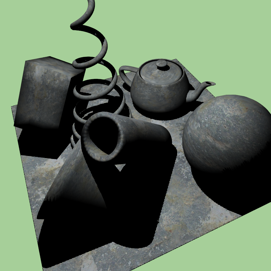
 Basic shadow maps
 Exponential variance shadow maps (with blur and anisotropic filtering)
The goal of this semester project was to implement variance shadow maps (VSM) as proposed by William Donnelly and Andrew Lauritzen [1] and its extension exponential variance shadow maps (EVSM) as proposed, again, by Andrew Lauritzen and Michael McCool in the article about layered variance shadow maps [2].
Algorithm
Variance Shadow Maps
The main idea of the base variance shadow map technique is to be able to use filtering functions on the shadow map texture such as mipmapping and anisotropic filtering. This is achieved through the usage of Chebyshev's inequality. Instead of storing depths in the shadow map, we store first and second moments - i.e. depth and squared depth. From these moments, we can compute the mean \( \mu = E(x) = M_1 \) and the variance \( \sigma^2 = E(x^2) - E(x)^2 = M_2 - M_1^2 \).
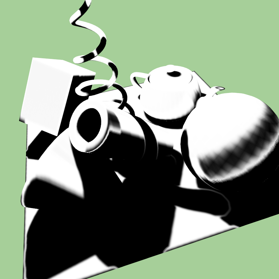
 VSM - anisotropic filtering off
 VSM - anisotropic filtering on
The Chebyshev's inequality gives us the upper bound of the amount of pixels that will be shadowed (i.e. shadow intensity of the fragment). The inequality is defined as: $$ P(x > t) \leq p_{max}(t) \equiv \frac{\sigma^2}{\sigma^2 + (t - \mu)^2} $$ One large disadvantage of this method is that it is prone to light bleeding since we only get the upper bound of the shadow intensity. Lower bound is unknown, which leads to unwanted and unnatural light areas, especially in penumbra of shadows that are cast onto different shadows. This can be partly resolved by clamping \( p_{max} \) by some minimum value. This reduces light bleeding but also reduces the quality of the shadows when set too high.
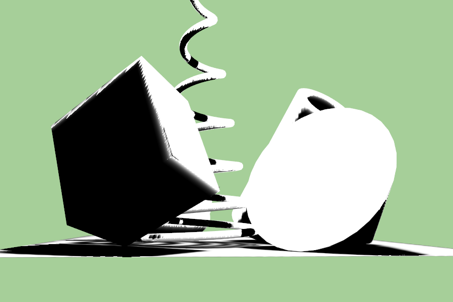
 Light bleeding (VSM without blur)
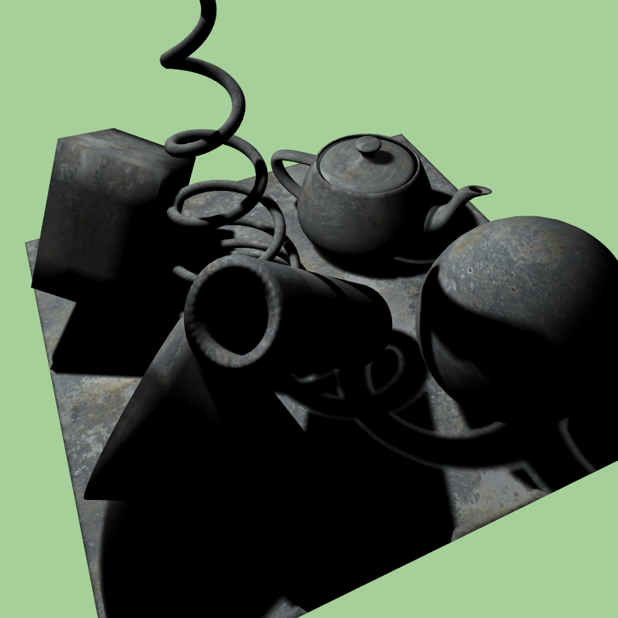 Light bleeding (VSM with blur)

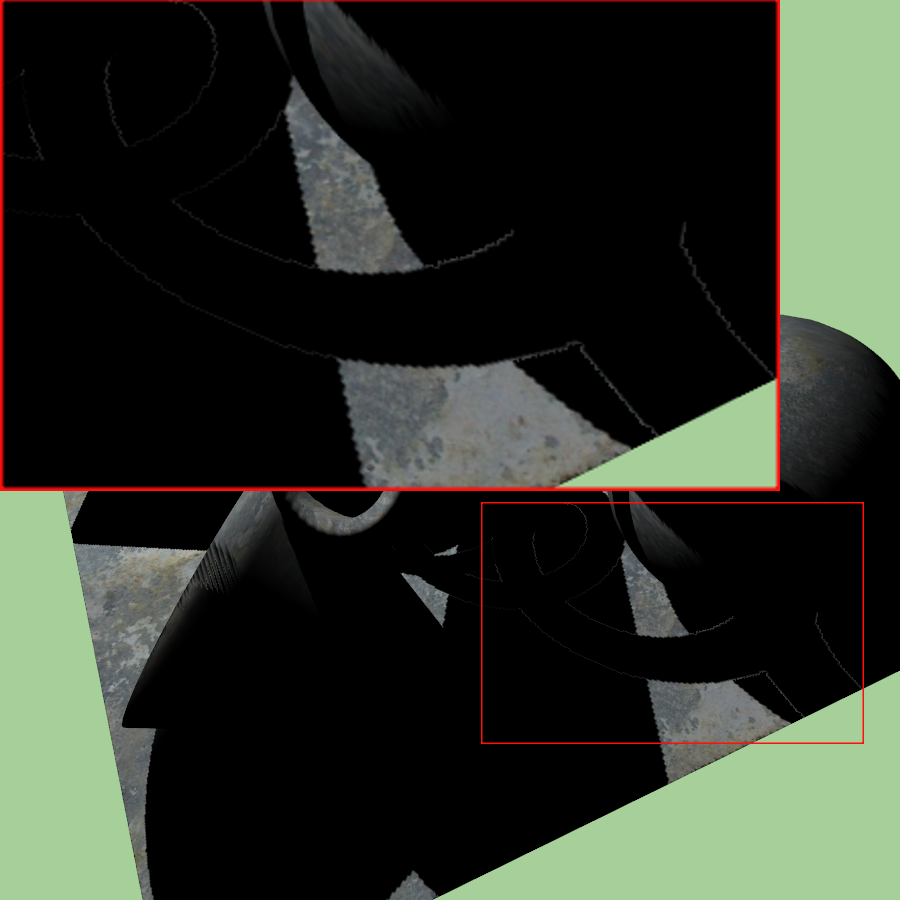
Naive light bleeding reduction for VSM. From left to right: 0.0 (no reduction), 0.3, 0.6. Note the artifacts on the edge of the ground plane (when blurring is used) that are mostly resolved using the main method - EVSM.
Layered Variance Shadow Maps
To solve the light bleeding issue, Lauritzen proposes decomposing the light space depth values into multiple layers using a linear warping function. For each layer \( L_i \) covering an interval \( [p_i, q_i] \), he defines a following warp: $$ \varphi_i(t) = \begin{cases} 0 & \text{if} \quad t \leq p_i \ \frac{t - p_i}{q_i - p_i} & \text{if} \quad p_i < t < q_i \ 1 & \text{if} \quad q_i \leq t \end{cases} $$ Furthermore, to avoid artefacts on layer boundaries, small overlap is suggested by the authors.
Exponential Variance Shadow Maps
As suggested at the end of the article by Lauritzen, the exponential warping function can also be used in tandem with layered variance shadow maps producing exponential variance shadow maps (EVSM). More specifically, we use two layers: the first layer contains a positive \( e^{cx}\) warp of the depth while the second contains a negative \( -e^{-cx} \) warp, where \( c \) is a constant and \( x \) is the depth. This means that in the texture we store first and second moments computed from these warped values.
As the title suggests, I've chosen to implement EVSM instead of multi-layered LVSM due to the fact that it produces shadows of better quality, uses less memory and is also less computationally expensive [2]. LVSM with 2 layers was implemented for comparison with EVSM, the splitting value and overlap of layers are manually configurable.
 LVSM with 2 layers and splitting value 0.93
 (manually set optimal value for the current scene view)
 EVSM (as opposed to LVSM, light bleed reduction works dynamically in all conditions)
Gaussian Blur
Since the VSM and its extensions LVSM and EVSM do not produce soft shadows we need to apply a gaussian blur to the depth map that we generated. This is correct (and encouraged) as opposed to regular shadow maps where blurring depths doesn't make sense.
For blurring we do two more passes using a single shader and two framebuffers (with two texture attachments). First pass is horizontal, second is vertical. Furthermore, in the case of 9x9 gaussian blur, I have implemented a linear approach to sampling texture, reducing the amount of taps (texture reads) from 9 to 5 as described in [3].
 EVSM with 256x256 resolution and no blur
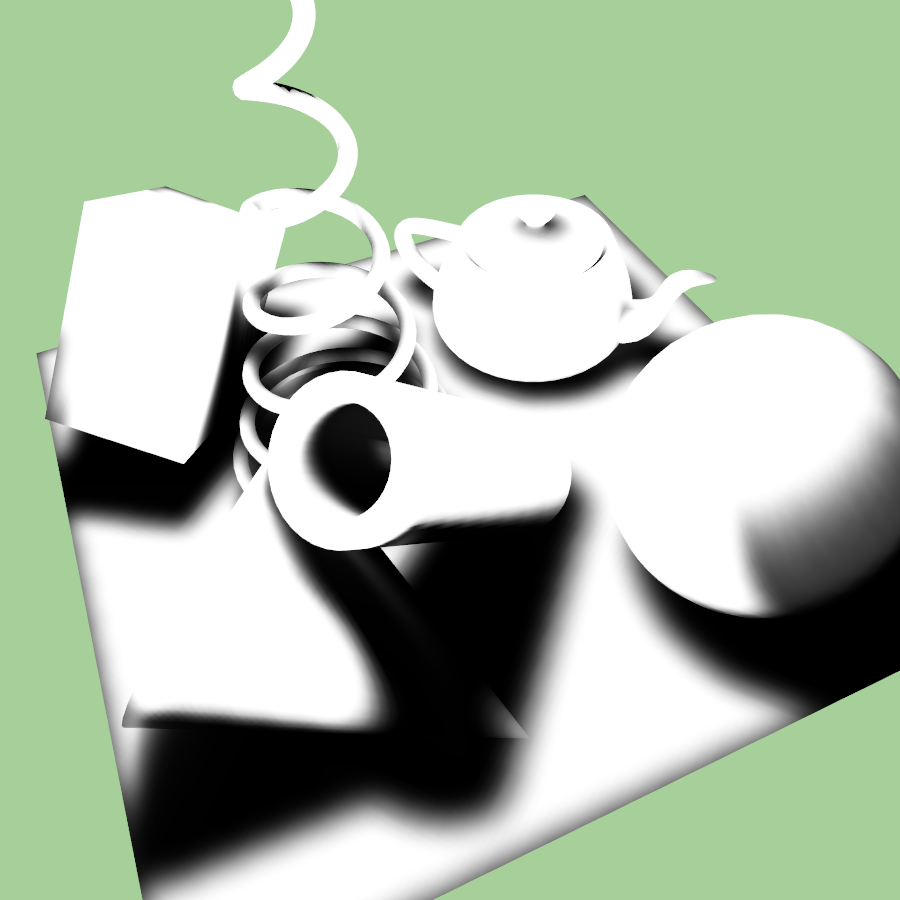 EVSM with 256x256 resolution and 9x9 blur
Comparison of some Implemented Methods
 Basic
Basic PCF 2x2 (HW using sampler2DShadow)
 PCF 3x3
 PCF 9x9
 VSM (no blurring)
 VSM with 3x3 PCF applied
 VSM with 9x9 blur
 EVSM (no blurring)
 EVSM (with 9x9 blur)
Implementation Details
Basic Shadow Maps
The implementation builds on the project that was provided for the course. The rendering of basic shadow maps and PCF shadow maps uses the shadow_mapping shaders that were implemented during the seminar. The basic shadow maps use the depth map texture (RGBA32F) and use non-projected coordinates for computation. The PCF 2x2 uses the g_ZBufferTexture (GL_DEPTH_COMPONENT) and sampler2DShadow to achieve quick hardware PCF. The manual implementations of PCF are computed with projected coordinates, textureOffset function is used instead of computing offsets (by texelSize) in shaders manually.
VSM
The VSM and EVSM methods have been created in separate shader programs for easier readability. In the first pass of VSM, we can simply save the moments in the shadow map. I have also implemented the formula that was, again, suggested by Andrew Lauritzen in GPU Gems [4] that reduces shadow bias and is described as: $$ M_2 = \mu^2 + \frac{1}{4} \Bigg( \bigg[ \frac{\partial t}{\partial x} \bigg]^2 + \bigg[ \frac{\partial t}{\partial y} \bigg]^2 \Bigg) $$
During the second pass we read these values and compute the variance and \( p_{max} \). We clamp the \( p_{max} \) with modifiable uniform u_LightBleedReduction. Optionally we can apply 3x3 PCF to find adjacent moments in the texture and compute average shadow intensity.
EVSM
The EVSM is similar, but instead of saving only two values in the first pass we need to store the exponentially warped depth moments. This means that we compute: $$ t_{positive} = \exp(c_x * t) $$ $$ t_{negative} = - \exp(-c_y * t) $$
where \( c_x \) and \( c_y \) are constants. In the article it holds that \( c_x = c_y \), but I decided to make them modifiable for easier testing.
During the second pass, we do the same as in VSM, but in this case for both positive and negative warp. We apply Chebyshev's inequality and select the smaller of the two results as the upper bound and therefore the final shadow intensity.
Gaussian Blur
I have implemented multiple blurring options for the application. All are selectable in the blur menu and applicable to the shadow maps. There are one pass implementations that naively sample all adjacent texels of the current texel. Then there are 5x5, 7x7 and 9x9 options that use a two pass algorithm which is viable due to the fact that gaussian blur kernel is a symmetrical matrix and therefore we can multiply each axis separately [5]. Furthermore, I have decided to optimize the blur shader with linear sampling as proposed in [3]. This means that we imitate GL_LINEAR sampling as opposed to GL_NEAREST as the author suggests. The linear sampling was implemented only for the 9x9 blur kernel. All the kernels were generated online using the gaussian kernel calculator [6] with the value of sigma set to 2.0.
Controls
The application can be controlled using the AntTweakBar user interface or with a multitude of shortcuts.
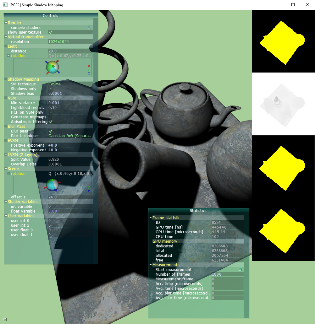 User interface of the application
- c - compile shaders
- s - show user textures
- d, D - decrease/increase shadow map resolution
- l, L - decrease/increase light distance from origin
- 0 - 9 - change shadow mapping technique
- S - show shadow only
- p - toggle PCF usage when VSM (only!) technique is used
- m - toggle generate mipmaps
- a - toggle anisotropic filtering
- g - toggle blur pass
- b, B - change blur function
- z, Z - change camera offset from origin
Measurements
Measurements were done on computer with these specifications:
- MS Windows 10 Home (64-bit), Version 1803, OS build 17134.407
- Intel Core i7-6700K Skylake CPU @ 4.00GHz 4.00GHz
- 32.0 GB RAM
- Nvidia GeForce GTX 1080
- OpenGL version 4.4
We can see from the table that the EVSM method provides very quick and good quality results when taking advantage of the optimized 9x9 gaussian blur implementation. The results are almost devoid of all light bleeding problems and general artifacts (such as incorrect ground edges when blur is applied to VSM). VSM and EVSM are comparable in speed. We can also notice that EVSM with filtering, mipmap generation (each frame for dynamic lights) and 9x9 blur is still 2x faster than naive 9x9 PCF implementation.
| Method | Basic (from seminar) |
PCF 2x2 (HW) |
PCF 3x3 |
PCF 3x3 (gaus.) |
PCF 9x9 (gaus.) |
VSM | VSM (3x3 PCF) |
VSM (9x9 blur) |
EVSM | EVSM (9x9 blur) |
EVSM (anis. filtering, mipmaps, 9x9 blur) |
|
|---|---|---|---|---|---|---|---|---|---|---|---|---|
| Avg. time \( [ \mu s]\) for 10000 frames |
2048x2048 | 425.65 | 311.96 | 584.14 | 591.03 | 3006.82 | 439.25 | 606.12 | 1172.04 | 459.16 | 1194.49 | 1687.53 |
| 1024x1024 | 218.19 | 183.72 | 257.43 | 258.03 | 1383.97 | 221.89 | 262.33 | 409.81 | 226.95 | 414.91 | 645.58 | |
| 512x512 | 160.27 | 149.02 | 168.90 | 168.45 | 924.27 | 160.23 | 170.19 | 214.94 | 162.51 | 217.22 | 365.93 | |
The blurring technique measurements show that the speed up from 1-pass to 2-pass algorithm is very significant as you can see in the difference between 5x5 and 5x5 (separated) columns. Furthermore, the usage of linear sampling for 9x9 blur provides us with identical results as for 5x5 discrete sampling since we need to do 5 taps in each axis for both methods, hence making the speedup also significant.
| Blur method | 3x3 | 5x5 | 5x5 (separ.) |
7x7 (separ.) |
9x9 (separ.) |
9x9 (separ., linear) |
|
|---|---|---|---|---|---|---|---|
| Avg. time \( [ \mu s]\) for 10000 frames |
1024x1024 | 146.46 | 380.14 | 185.11 | 237.67 | 292.52 | 186.19 |
Download
- Executable (Requires OpenGL 4.0)
References
- William Donnelly & Andrew Lauritzen, Variance Shadow Maps, Proceedings of the 2006 Symposium on Interactive 3D Graphics and Games, 2006, ISBN: 1-59593-295-X, pages 161-165, available at: http://www.punkuser.net/vsm/vsm_paper.pdf
- Andrew Lauritzen & Michael McCool, Layered Variance Shadow Maps, Proceedings of Graphics Interface 2008, ISBN: 978-1-56881-423-0, pages 139-146, available at: http://www.punkuser.net/lvsm/lvsm_web.pdf
- Daniel Rákos, Efficient Gaussian Blur with Linear Sampling, [online], available at: http://rastergrid.com/blog/2010/09/efficient-gaussian-blur-with-linear-sampling/
- Andrew Lauritzen, Summed-Area Variance Shadow Maps, [online], available at: https://developer.nvidia.com/gpugems/GPUGems3/gpugems3_ch08.html
- Bert (user), How is Gaussian Blur Implemented?, [online], available at: https://computergraphics.stackexchange.com/questions/39/how-is-gaussian-blur-implemented
- Undisclosed author, Gaussian Kernel Calculator, [online], available at: http://dev.theomader.com/gaussian-kernel-calculator/
- HTML Table Generator, [online], available at: https://www.tablesgenerator.com/html_tables